Traffic prediction based on public transport transit times (IV): Visualization
by
Yet another entry on the project about traffic prediction (online here: http://fergonco.org/border-rampage/).
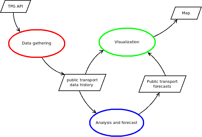
In the previous post I showed how the data was analyzed and the forecasts produced. In this one I will show how the map shows all this information. This is the last of the three processes of the data flow diagram, the one in green:
In order to draw gathered and forecast data they have to be unified in a single dataset that the mapping software, GeoServer, can process. For gathered data this involves some transformation, which was done with SQL views. In the case of forecast data, it does not require any transformation but it has to be generated regularly. The next points will show:
- How gathered data is transformed.
- How forecast data is generated.
- How GeoServer draws the unified dataset.
Transforming gathered data
In order to show how the data is transformed I will first describe (again, if you have read the previous posts) how the data is stored in the database. Then I will show how the data should be so that GeoServer is able to consume it.
Database model
I will start by recalling quickly how the public transport network is stored in the database. For brevity, some details are omitted. Refer to the previous blog post to see the complete explanation.
The following diagram shows the relevant database model.
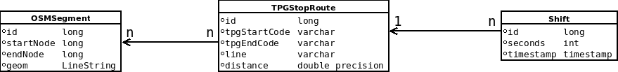
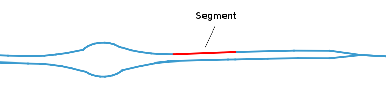
There is have a table with segments, OSMSegment, which contains the segments that are part of the public transport network:
 id | startnode  |  endnode   |                         geom
----+------------+------------+-------------------------------------------------------
  1 | 3735051668 |  429658525 | LINESTRING(6.1413701 46.2103922,6.1415854 46.2105857)
  2 |  768498823 | 3606163490 | LINESTRING(6.1408597 46.2098549,6.1409013 46.2099104)
  3 | 3606163601 | 1549433399 | LINESTRING(6.1410869 46.210142,6.141181 46.2102227)
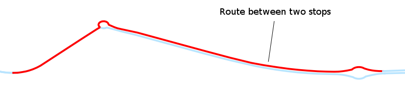
This OSMSegments are referenced by records in TPGStopRoute, which contains an entry for each pair of consecutive stops of a service line and references the OSMSegments that compose the route between these two stops.
 id  | line | starttpgcode | endtpgcode |     distance
-----+------+--------------+------------+-------------------
  72 | Y    | POLT         | PAGN       | 0.747157007209657
 103 | F    | LMLD         | ZIMG       | 0.685551031729394
 104 | F    | ZIMG         | LMLD       | 0.685551031729394
Finally, the data gathered is stored in the Shift table, that contains the time elapsed between stops and the reference to the TPGStopRoute.
   id   | seconds |  sourceshiftid  |   timestamp   | vehicleid | route_id
--------+---------+-----------------+---------------+-----------+----------
 188508 |      77 | 1-4-2017+185220 | 1493643974000 | 185220    |      103
 188509 |     144 | 1-4-2017+185221 | 1493644119000 | 185221    |      105
 188510 |     112 | 1-4-2017+185222 | 1493644231000 | 185222    |      107
Summarizing: Shifts reference TPGStopRoutes, which reference OSMSegments.
Now, how should the data be in order to be drawn from GeoServer?
GeoServer temporal dimension
The aim is to have a map showing segments of the public transport network painted with a color depending on the speed of the last vehicle passage. And this for several time coordinates (instants) that the user can select on the web application. In order to fulfill these requirements, GeoServer needs a dataset with the following fields:
- A geometry field with the geometry to draw, in this case a segment of the public transport network.
- A speed field with the speed of the bus through the segment, in order to choose the corresponding color.
- A timestamp field with the exact timestamp when this record exists (GeoServer offers other possibilities but this one is the one I used).
GeoServer uses the last field to filter the dataset and get only the features that exist on the selected time coordinate. This means that, for every time coordinate that the user can select, there must be a subset of the dataset whose timestamp field is equal to this time coordinate. This subset will contain the data necessary to draw the map in the selected time coordinate.
Thus, if a segment has the same speed in two consecutive time coordinates, there will be two records that are identical except for the timestamp field. Seen from another perspective: the dataset must contain the data for the maps at every possible time coordinate, and will have a timestamp field that allows GeoServer to filter out the data that is not relevant for the time coordinate selected by the user.
I had to make some critical decisions here: what are the time coordinates I want to offer the user? Do I want to let him navigate several months of data history? Additionally, what would be the resolution of the time dimension? Each time a bus arrived to a stop? Each quarter of hour? These questions (time dimension range and resolution) are critical because with the amount of data involved they can greatly complicate the implementation. The very conservative decision I made was: each quarter of hour for the last 24 hours.
Transformation
I have shown how the database is organized and how the data must be in order to be consumed by GeoServer. Now I will explain how the transformation was done by means of SQL views.
A first view joins Shift, TPGStopRoute and OSMSegment in order to get speeds and geometries on the same table. This yields a result where each Shift is replicated as many times as there are segments in the associated TPGStopRoute, each of this replicas having a different segment geometry. I called this a GeoShift.
Then, another view has the timestamps that correspond to “the last 24 hours each quarter of hour” whenever it is computed.
These two views are joined producing a result that for each timestamp there is a record for each segment having: the timestamp, the segment geometry and the most recent Shift speed before the timestamp. The result of this join can be used by GeoServer as it contains the segment geometry, the speed and the timestamp to filter the table.
Note that the timestamps view would run outdated as times goes by so there is a process in the server that refreshes the views.
This implementation faces some performance limitations:
-
The final result contains a record for each segment and for each timestamp. In the reduced area the project focuses on there are 4000 segments. On the other side, “the last 24 hours each quarter of hour” produces 96 timestamps. The result for this limited area and time dimension is 384000 records. It is not a big deal to serve a map with this amount of data but one can easily see that it does not escalate. Specially, as we deal with bi-dimensional data, focusing on bigger area would increase quadratically the number of segments.
-
Without going into the query details, joining the timestamps views and the Shifts involves a subquery, which is quite inefficient. After installing all the indexes and being sure PostgreSQL uses them, the whole process takes between 1 and 2 minutes. Probably the “views” approach is wrong in itself and an incremental solution that updates the drawing dataset each time new data is gathered would be much lighter computationally.
Forecast data
As gathered data, forecast data is generated for each quarter of hour for the next 24 hours.
The table where forecasts are stored has already the structure required by GeoServer: a geometric field, speed and a timestamp.
The process of populating the forecast table is like this:
- For each segment.
- Get the statistical model from the database (this is dealt with in detail in the previous post).
- For each quarter of hour in the next 24 hours.
- Gather variable values: weather, holidays, day of the week, timestamp, …
- Make a forecast using the segment model.
- Store the forecast in the forecast table.
Visualization
Finally, in order to get a unique dataset, a view performs a SQL union between the tables containing the gathered data and the forecast data.
This result can be loaded in GeoServer. The only two special configurations it requires are:
- The timestamp field is configured in the “Dimensions” tab.
- The symbology is configured to show the four different speed categories with rules like this one:
	<Rule>
	  <Name>Rule20_30</Name>
	  <Title>[20, 30[</Title>
	  <ogc:Filter>
		<ogc:And>
		  <ogc:PropertyIsGreaterThanOrEqualTo>
			<ogc:PropertyName>speed</ogc:PropertyName>
			<ogc:Literal>20</ogc:Literal>
		  </ogc:PropertyIsGreaterThanOrEqualTo>
		  <ogc:PropertyIsLessThan>
			<ogc:PropertyName>speed</ogc:PropertyName>
			<ogc:Literal>30</ogc:Literal>
		  </ogc:PropertyIsLessThan>
		</ogc:And>
	  </ogc:Filter>
	  <LineSymbolizer>
		<Geometry>
		  <ogc:PropertyName>geom</ogc:PropertyName>
		</Geometry>
		<Stroke>
		  <CssParameter name="stroke">#ffba00</CssParameter>
		  <CssParameter name="stroke-width">4</CssParameter>
		</Stroke>
		<PerpendicularOffset>4</PerpendicularOffset>
	  </LineSymbolizer>
	</Rule>
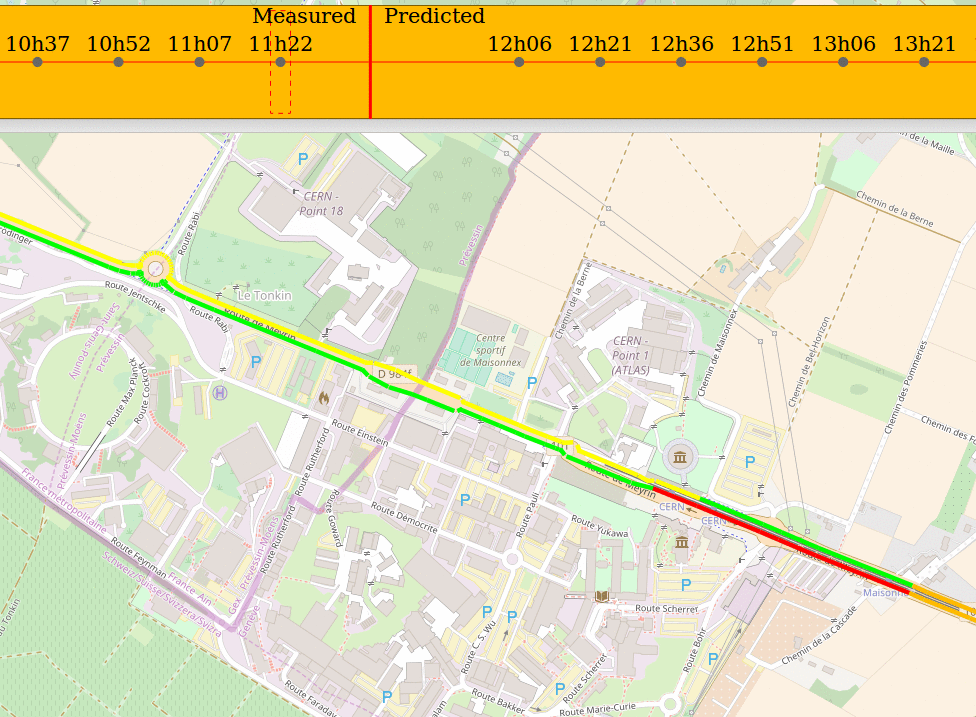
Note the use of PerpendicularOffset to symbolize the line on one side of the geometry, allowing thus to differentiate both segment directions.
UPDATE:
… and here you have an image of the result.